This post is part of the What Is… series that explains spatial audio techniques and terminology.
Spatial hearing is how we are able to locate the direction of a sound source. This is generally split in to azimuth (left/right) and elevation (vertical) localisations. Knowing how we localise is essential to understanding the spatial audio technologies. Human spatial hearing is a complex topic with lots of subtleties so we’ll ease in with some of the main concepts.
Interaural Time Difference (ITD)
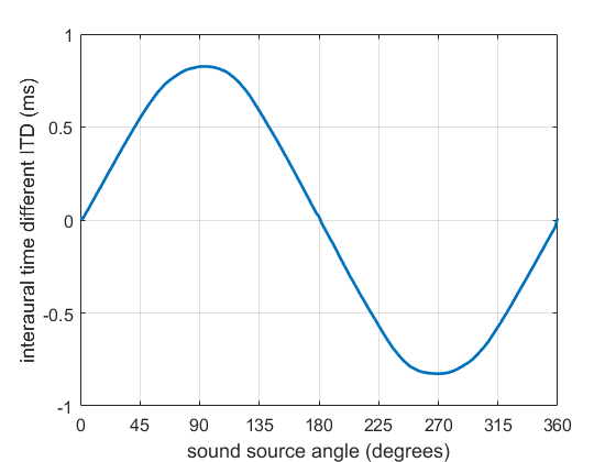
Consider a single sound source near to a listener. The sound source will radiate sound waves that will travel through the air to listener. These waves will reach the nearer (ipsilateral) ear of the listener earlier than the further (contralateral). This produces a time difference between the signals at both eardrums known as the interaural time difference (ITD). The brain can extract the time difference by comparing the two signals and will use this as an estimate of the direction of the sound. Whichever ear is leading in time dictates whether the sound is heard to the left or the right. The graph shows the average ITD for frequencies up to 1400 Hz. It has a clear sinusoidal shape that varies predictably with azimuth, making it a useful localisation cue.
ITD cues are mainly evaluated at low frequencies (below approximately 1400 Hz). This is the frequency range at which the wavelength of the sound is long enough when compared to the size of the head to avoid phase ambiguity. Above this frequency the phase can “wrap” around and it not possible to tell if there have been, say, 0.5 cycles, 1.5 cycles etc.
Luckily, we can use another method to localise in higher frequencies.
Interaural Level Difference (ILD)
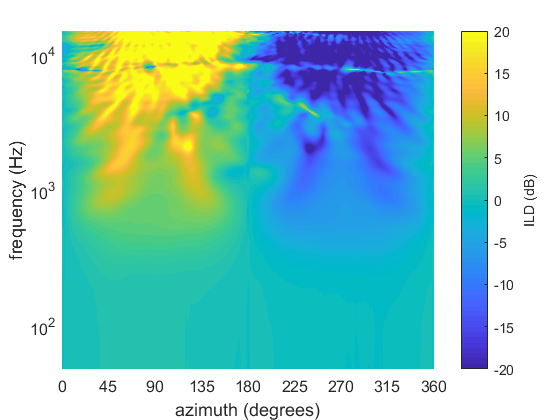
As frequency increases and the wavelength becomes shorter than the size of the listener’s head, acoustic shadowing becomes important, producing an interaural level difference (ILD). The shadowing causes the level at the contralateral ear to be reduced compared to the ipsilateral. This is in contrast to low frequencies where the wavelengths are so large that the level differences to not vary significantly with source direction (unless the sound source is very close!).
Where ITD exhibits a sinusoidal shape, making direction estimation relatively simple, ILD can vary in a complex manner with source direction. This is due to how the sound waves interact with the head and doesn’t mean that the biggest level difference happens as \(pm90^circ\). In fact, this ILD is actually lower at \(pm90^circ\) than at some less lateral positions. This is known as the acoustic bright spot. The complex ILD patterns are shown in the graph where the more yellow/blue the colour the larger the ILD. Yellow means the left ear is greater than the right and blue the right is greater than the left.
ITD and ILD are work well for differentiating between left and right. But imagine a sound source starts directly infront of you, moves in an arc over your head to finish directly behind you. At no point do ITD and ILD have any value other than zero but we can still perceive the elevation of the sound source. How are we able to do this?
Spectral Cues
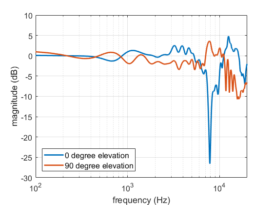
The outer ears (pinnae) are a very complex shape. They cause the sounds to be filtered in a way that is highly direction dependent. This leads to peaks and notches in the frequency response of the source spectrum that can be used to evaluate the direction, primarily for elevation. The frequencies of the peaks and notches are highly individual, depending strongly on the shape of the outer ears. This is something that the brain learns and it can use this internal template to incoming sounds and give an estimate of localisation.
For example, the graph to the left shows the frequency spectra for a sound source at two different positions: in front and above. The frontal source has a deep notch at 8 kHz which is not the case for the elevated source. This could be used to differentiate between the two elevations, even though the signals at the left and right ears would be (nearly) identical.
Localisation accuracy tends to be much less accurate for elevation than it is for azimuthal (left/right) judgements. This can have implications for how we might design a spatial audio system or on how well they can work.
Is that it?
Not by a long shot! We haven’t covered things like interaural envelope difference, distance estimation, the effect of head movement, the precedence effect, the ventriloquist effect but these are the main principles we need to understand to get to grips with the basics of spatial audio.