What Is... Archives • SSA Plugins

Posted on 18th July 201724th September 2018 by Peter

What Is… Higher Order Ambisonics?

This post is part of a What Is… series that explains spatial audio techniques and terminology.

The last post was a brief introduction to Ambisonics covering some of the main concepts of first-order Ambisonics. Here I’ll give an overview of what is meant by Higher Order Ambisonics (HOA). We’ll be sticking to the more practical details here and leaving the maths and sound field analysis for later.

Higher Order Ambisonics (HOA) is a technique for storing and reproducing a sound field at a particular point to an arbitrary degree of spatial accuracy. The degree of accuracy to which the sound field can be reproduced depends on several elements: the number of loudspeakers available at the reproduction stage, how much storage space you have, computer power, download/transmission limits etc. As with most things, the more accuracy you want the more data you need to handle.

Encoding

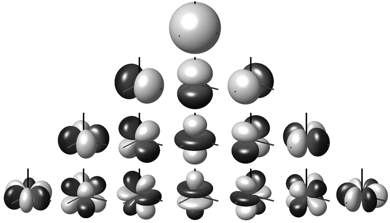
Spherical harmonics used for third-order HOA (image by Dr Franz Zotter https://commons.wikimedia.org/wiki/File:Spherical_Harmonics_deg3.png)

In its most basic form, HOA is used to reconstruct a plane wave by decomposing the sound field into spherical harmonics. This process is known as encoding. Encoding creates a set of signals that depend on the position of the sound source, with the channels weighted depending on the source direction. The functions become more and more complex as the HOA order increases. The spherical harmonics are shown in the image up to third-order. These third-order signals include, as a subset, the omnidirectional zeroth-order and the first-order figure-of-eights. Depending on the source direction and the channel, the signal can also have its polarity inverted (the darker lobes).

An infinite number of spherical harmonics are needed to perfectly recreate the sound field but in practice the series is limited to a finite order \(M\). An ambisonic reconstruction of order \(M > 1\) is referred to as Higher Order Ambisonics (HOA).

An HOA encoded sound field requires \((M+1)^{2}\) channels to represent the scene, e.g 4 for first-order, 9 for second, 16 for third, etc. We can see that very quickly we require a very large number of audio channels even for relatively low orders. However, as with first-order Ambisonics, it is possible to do rotations of the full sound field relatively easily, allowing for integration with head tracker information for VR/AR purposes. The number of channels remains the same no matter how many sources we include. This is a great advantage for Ambisonics.

Decoding

The sound field generated by order 1, 3, 5 and 7 Ambisonics for a 500 Hz sine wave. The black circle in the middle is approximately the size of a listener’s head.

The encoded channels contain the spatial information of the sound sources but are not intended to be listened to directly. A decoder is required that converts the encoded signals to loudspeaker signals. The decoder has to be designed for your particular listening arrangement and takes into account the positions of the loudspeakers. As with first-order Ambisonics, regular layouts on a circle or sphere provide the best results.

The number of loudspeakers required is at least the number of HOA encoded channels coming in.

A so-called Basic decoder provides a physical reconstruction of the sound field at the centre of the array. The size of this physically accurately reconstructed area increases with increasing order but decreases with frequency. Low frequency ranges can be reproduced physically (holophony) but eventually the well-reproduced region becomes smaller than the size of a human head and decoding is generally switched to a max rE decoder, which is designed to optimise psychoacoustic cues.

The (slightly trippy) animation shows orders 1, 3, 5 and 7 of a 500 Hz sine wave to demonstrate the increasing size of the well-reconstructed region at the centre of the array. All of the loudspeakers interact to recreate the exact sound field at the centre but there is some unwanted interference out of the sweet spot.

Why HOA?

Since the number of loudspeakers has to at least match the number of HOA channels the cost and practicality are often the main limiting factor. How many people can afford 64 loudspeakers needed for a 7th order rendering? So why bother encoding things to a high order if we are limited to lower order playback? Two reasons: future-proofing and binaural.

First, future-proofing. One of the nice properties of HOA is that you can select a subset of channels to use for a lower order rendering. The first four channels in a fifth-order mix are exactly the same as the four channels of a first-order mix (see the spherical harmonic images above). We can easily ignore the higher order channels without having to do any approximative down-mixing. By encoding at a higher order than might be feasible at the minute you can remain ready for a future when loudspeakers cost the same as a cup of coffee (we can dream, right?)!

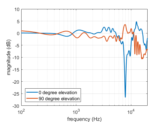
Second, binaural. If the limiting factors to HOA are cost and loudspeaker placement issues then what if we use headphones instead? A binaural rendering uses headphones to place a set of virtual loudspeakers around the listener. Now our rendering is only limited by the number of channels our PC/laptop/smartphone can handle at any one time (and the quality of the HRTF). The aXMonitor is an example of an Ambisonics-to-binaural decoder that can be loaded into any DAW that accepts VST format plugins, plug Pro Tools | Ultimate in AAX format.

The Future

As first-order Ambisonics makes its way into the workflow of not just VR/AR but also music production environments, we’re already seeing companies preparing to introduce HOA. Facebook already includes a version of second-order Ambisonics in its Facebook 360 Spatial Workstation [edit: They are now up to third order!]. Google have stated that they are working to expand beyond first-order for YouTube. I have worked with VideoLabs to include third-order Ambisonics in VLC Media player. This is in the newest version of VLC.

Microphones for recording higher than first-order aren’t at the stage of being accessible to everyone yet, but there are tools, like the a7 Ambisonics Suite that will let you encoded mono signals up to seventh-order, as well as to process the Ambisonics signal. There are also up-mixers like Harpex if you want to get higher orders from existing first-order recordings.

All of this means that if you can encoded your work in higher orders now, you should. You do not want to have to go back to your projects to rework them in six months or a year when you can do it now.

Posted on 27th June 201724th September 2018 by Peter — 4 Comments

What Is… Ambisonics?

This post is part of a What Is… series that explains spatial audio techniques and terminology.

Ambisonics is a spatial audio system that has been around since the 1970s, with lots of the pioneering work done by Michael Gerzon. Interest in Ambisonics has waxed and waned over the decades but it is finding use in virtual, mixed and augmented reality because it has a number of useful mathematical properties. In this post you’ll find a brief summary of first-order Ambisonics, without going too deeply into the maths that underpins it.

Unlike channel-based systems (stereo, VBAP, etc.) Ambisonics works in two stages: encoding and decoding. The encoding stage converts the signals into B-format (spherical harmonics), which are agnostic of the loudspeaker arrangement. The decoding stage takes these signals and converts them to the loudspeaker signals needed to recreate the scene for the listeners.

Ambisonic Encoding

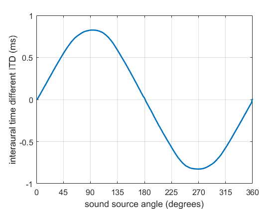
First-order Ambisonic encoding to SN3D for a sound source rotating in the horizontal plane. The Z channel is always zero for these source directions.

A mono signal can be encoded to Ambisonics B-format using the following equations:

\(\begin{eqnarray}
W &=& S \\
Y &=& S\sin\theta\cos\phi \\
Z &=& S\sin\phi\\
X &=& S\cos\theta\cos\phi
\end{eqnarray}
\)

where \(S\) is the signal being encoded, \(\theta\) is the azimuthal direction of the source and \(\phi\) is the elevation angle. (These equations use the semi-normalised 3D (SN3D) scheme, as in the AmbiX format used by Google for YouTube. The channel ordering also follows the AmbiX standard.) First-order Ambisonics can also be captured using a tetrahedral microphone array.

B-format is a representation of the sound field at a particular point. Each sound source is encoded and the W, X, Y and Z channels for each source are summed to give the complete sound field. Therefore, no matter how many sound sources are in the scene, only 4 channels are required for transmission.

This encoding can be thought of as capturing a sound source using one omnidirectional microphone (W) and 3 figure-of-eight microphones pointing along the Cartesian x-, y- and z-axes. As shown in the animation to the side, the amplitude of the W channel stays constant for all source positions while the X and Y channels change relatives gains and sign (positive/negative) with source position. Comparison of the polarity of X and Y with W allows the direction of the sound source to be derived.

Ambisonic Decoding

Decoding is the process of taking the B-format signals and converting them to loudspeaker signals. Depending on the loudspeaker layout this can be relatively straightforward or really quite complex. In the most simple cases, with a perfectly regular layout, the B-format signals are sampled at the loudspeaker positions. Other methods, (for example, mode-matching or energy preserving) can be used but tend to give the same results for a regular array.

Assuming a regular array and good decoder, an Ambisonic decoder will recreate the exact sound field up to approximately 400 to 700 Hz. Below this limit frequency the reproduction error is low and the ITD cues are well recreated, meaning the system can provide good localisation. Above this frequency the recreated sound field deviates from the intended physical sound field so some psychoacoustic optimisation is applied. This is realised by using a different decoder in higher frequency ranges that focusses the energy in as small a region as possible in the loudspeaker array. This helps produce better ILD cues and a more precise image.

Ambisonics differs from VBAP because, in most cases, all loudspeakers will be active for any particular source direction. Not only will the amplitude vary, the polarity of the loudspeaker signals will also matter. Ambisonics uses all of the loudspeakers to “push” and “pull” so that the correct sound field is recreated at the centre of the loudspeaker array.

What is a Good Decoder?

A “good” Ambisonic decoder requires an appropriate loudspeaker arrangement. Ambisonics ideally uses a regularly positioned loudspeaker arrangement. For example, a horizontal-only system will place the loudspeakers at regular intervals around the centre of an array.

Any number of loudspeakers can be used to decode the sound scene but using more than required can lead to colouration problems. The more loudspeakers are added the more of a low-pass filtering effect there is for listeners in the centre of the array. So what is the best number of loudspeakers to use for first-order Ambisonics? It is generally agreed that 4 loudspeakers placed in a square be used for a horizontal system and 8 in a cuboid be used for 3D playback. This avoids too much colouration and satisfies several conditions for good (well… consistent) localisation.

There are metrics defined in the Ambisonics literature that predict the quality of the system in terms of localisation. These are the velocity and energy vectors and they are deserving of their own article. For now, it’s worth noting that the velocity vector links to low-frequency ITD localisation cues. Decoders are designed to optimise it at low-frequencies while they are optimised using the energy vector at higher frequencies. The high frequency decoder is known as a ‘max rE’ decoder, so-called because it aims to maximise the magnitude of the energy vector metric. This is just another way of saying that the energy is focussed in as small an area as possible.

Ambisonic Rotations

When it comes to virtual and augmented reality, efficient rotation of the full sound field is to follow head movements is a big plus. Thankfully, Ambisonics has got us covered here. The full sound field can be rotated before decoding by blending the X, Y and Z channels correctly.

The advantage of rotating the Ambisonic sound field is that any number of sound sources can be encoded in just 4 channels, meaning rotating a sound field with one sound source takes as much effort as rotating one with 100 sound sources.

That’s the basics of Ambisonics covered. At some point we’ll look more at measures of quality of Ambisonics decoders and how well ITD and ILD are recreated. This blog has also only covered first-order Ambisonics, but Higher Order Ambisonics (HOA) is likely make its way to VR platforms in a significant way in the near future so I’ll cover that soon.

Do you have any spatial audio questions you’d like to have answered? Just leave a comment and let me know!

Posted on 22nd June 2017 by Peter

What Is… Stereophony?

This post is part of my What Is… series that explains spatial audio techniques and terminology.

OK, you know what stereo is. Everyone knows what stereo is. So why bother writing about it? Well, because it allows us to introduce some links between the reproduction system and spatial perception before moving on to systems which use much more than 2 loudspeakers.

Before going any further, this post will deal with amplitude panning. Time panning will be left for another day. I also won’t be covering stereo microphone recording techniques because that could fill up its own series of posts.

The Playback Setup

A standard stereo setup is two loudspeakers placed symmetrically at \(\pm30^{\circ}\) to the left and right of the listener. We will assume for now that there is only a single listener equidistant from both loudspeakers. The loudspeaker basis angle can be wider or narrower but if they get too wide there is a hole-in-the-middle problem. Too narrow and we reduce the range of positions at which the source can be placed. Placing the loudspeakers at \(\pm30^{\circ}\) gives a good compromise between these two, balancing sound image quality with potential soundstage width.

A standard stereo listening arrangement.

The tangent law prediction of perceived source angle for different level differences

Placing the Sound

Amplitude panning takes a mono signal and sends copies to the two output channels with (potentially) different levels. When played back over two loudspeakers the level difference between the two channels controls the perceived direction of the sound source. With amplitude panning the perceived image will remain between the loudspeakers. If we know the level difference between the two channels then we can predict the perceived direction using a panning law. The two most famous of these are the tangent law and the sine law. The tangent law is defined as
\begin{equation}
\frac{\tan\theta}{\tan\theta_{0}} = \frac{G_{L} – G_{R}}{G_{L} + G_{R}}
\end{equation}
where \(\theta\) is the source direction, \(\theta_0\) is the angle between either loudspeaker and the front (30 degrees in the case illustrated above) and \(G_{L}\) and \(G_{R}\) are the linear gains of the left and right loudspeakers.

The ITD produced for a source panned with loudspeaker level differences generated by the tangent law.

How It Works

Despite being simple conceptually and very common, the psychoacoustics of stereo are actually quite complex. We’ll stick to discussing how it relates to the main spatial hearing cues.

As long as both loudspeakers are active, signals from both loudspeakers will reach both ears. Due to the layout symmetry, both ears receive signals at the same time but with different intensities corresponding to the level differences of the loudspeakers. Furthermore, since it has further to travel, the signal from the left loudspeaker will reach the right ear slightly later than the signal from the right loudspeaker. The opposite is true for the right ear. This time difference combined with the intensity difference gives rise to interference that generates phase differences at the ears. These phase differences are interpreted as time differences, moving the sound between the loudspeakers.

The ITD (below 1400 Hz) is shown in the figure and is roughly linear with panning angle. This is pretty close to exactly what we see for a real sound source moving between these angles. This works pretty well for loudspeakers at \(\pm30^{\circ}\) or less, but once the angle gets bigger the relationship becomes slightly less linear.

These strong, predictable ITD cues mean that any sound source with a decent amount of low frequency information will allow us to place the image pretty precisely. Content in higher frequency ranges won’t necessarily be in the same direction as long frequency content because ILD becomes the main cue.

Even though stereo gives rise to interaural differences that similar to those of a real source, that does not mean it is a physically-based spatial audio system (like HOA and WFS). The aim is to produce a psychoacoustically plausible (or at least pleasing) sound scene. Psychoacoustically-based spatial audio systems tend to use the loudspeakers available to fit some aim (precise image, broad source) without regards to if the resulting sound scene ressembles anything a real sound source would emit.

So, there you have a quick overview of stereo from a spatial audio perspective. There are other issues that will be cover later because they relate to other spatial audio techniques. For example, what if I’m not in the sweet spot? What if the speakers are to the side or I turn my head? What if I add a third (or forth or fifth) active loudspeaker? Why do some sounds panned to the centre sound elevated? All of these remaining and non-trivial points shows just how complex perception of even a simple spatial audio system can be.

Posted on 20th June 201724th September 2018 by Peter

What Is… Spatial Hearing?

This post is part of the What Is… series that explains spatial audio techniques and terminology.

Spatial hearing is how we are able to locate the direction of a sound source. This is generally split in to azimuth (left/right) and elevation (vertical) localisations. Knowing how we localise is essential to understanding the spatial audio technologies. Human spatial hearing is a complex topic with lots of subtleties so we’ll ease in with some of the main concepts.

Interaural Time Difference (ITD)

ITD for a Neumann KU100 dummy head averaged across all frequencies below 1400 Hz

Consider a single sound source near to a listener. The sound source will radiate sound waves that will travel through the air to listener. These waves will reach the nearer (ipsilateral) ear of the listener earlier than the further (contralateral). This produces a time difference between the signals at both eardrums known as the interaural time difference (ITD). The brain can extract the time difference by comparing the two signals and will use this as an estimate of the direction of the sound. Whichever ear is leading in time dictates whether the sound is heard to the left or the right. The graph shows the average ITD for frequencies up to 1400 Hz. It has a clear sinusoidal shape that varies predictably with azimuth, making it a useful localisation cue.

ITD cues are mainly evaluated at low frequencies (below approximately 1400 Hz). This is the frequency range at which the wavelength of the sound is long enough when compared to the size of the head to avoid phase ambiguity. Above this frequency the phase can “wrap” around and it not possible to tell if there have been, say, 0.5 cycles, 1.5 cycles etc.

Luckily, we can use another method to localise in higher frequencies.

Interaural Level Difference (ILD)

As frequency increases and the wavelength becomes shorter than the size of the listener’s head, acoustic shadowing becomes important, producing an interaural level difference (ILD). The shadowing causes the level at the contralateral ear to be reduced compared to the ipsilateral. This is in contrast to low frequencies where the wavelengths are so large that the level differences to not vary significantly with source direction (unless the sound source is very close!).

Where ITD exhibits a sinusoidal shape, making direction estimation relatively simple, ILD can vary in a complex manner with source direction. This is due to how the sound waves interact with the head and doesn’t mean that the biggest level difference happens as \(\pm90^\circ\). In fact, this ILD is actually lower at \(\pm90^\circ\) than at some less lateral positions. This is known as the acoustic bright spot. The complex ILD patterns are shown in the graph where the more yellow/blue the colour the larger the ILD. Yellow means the left ear is greater than the right and blue the right is greater than the left.

ITD and ILD are work well for differentiating between left and right. But imagine a sound source starts directly infront of you, moves in an arc over your head to finish directly behind you. At no point do ITD and ILD have any value other than zero but we can still perceive the elevation of the sound source. How are we able to do this?

Spectral Cues

The frequency spectra for a sound source directly in front of and above the listener. Note the significant notch at 8 kHz for the frontal source that is missing in the elevated source.

The outer ears (pinnae) are a very complex shape. They cause the sounds to be filtered in a way that is highly direction dependent. This leads to peaks and notches in the frequency response of the source spectrum that can be used to evaluate the direction, primarily for elevation. The frequencies of the peaks and notches are highly individual, depending strongly on the shape of the outer ears. This is something that the brain learns and it can use this internal template to incoming sounds and give an estimate of localisation.

For example, the graph to the left shows the frequency spectra for a sound source at two different positions: in front and above. The frontal source has a deep notch at 8 kHz which is not the case for the elevated source. This could be used to differentiate between the two elevations, even though the signals at the left and right ears would be (nearly) identical.

Localisation accuracy tends to be much less accurate for elevation than it is for azimuthal (left/right) judgements. This can have implications for how we might design a spatial audio system or on how well they can work.

Is that it?

Not by a long shot! We haven’t covered things like interaural envelope difference, distance estimation, the effect of head movement, the precedence effect, the ventriloquist effect but these are the main principles we need to understand to get to grips with the basics of spatial audio.

Posted on 16th June 201718th November 2017 by Peter

What Is… Spatial Audio?

This post is the first in a What Is… series. The idea is to explain different techniques, terminology and concepts related to spatial audio. This will range from the most common terms right through to some more obscure topics. And where better to start than “spatial audio” even means!

Spatial audio (with some exceptions) has generally been confined to academia but is rapidly finding applications in virtual reality (VR). There are even moves to bring it to broadcasting so it can be enjoyed by people in the comfort of their living rooms. As spatial audio moves from labs to living rooms it is worth exploring all of the different techniques that have been developed up to this point.

However, defining spatial audio can quickly become rather philosophical. For example, is a mono recording spatial audio? If I take a single microphone to a concert hall and record a performance then I have captured the sense of space, through echoes and reverberation, not just the performances themselves. This means that the space is encoded into the signal – we can tell if a recording is made in a dry studio or a cathedral. For the purposes of this series I will not be considering this to be spatial audio. Instead, I will be defining spatial audio as any audio encoding or rendering technique that allows for direction to be added to the source. How well this is reproduced to the listener will depend on the encoding and playback system but, in general, a spatial audio system will allow different sounds placed in different positions to be directionally differentiated.

There are a large number of different spatial audio techniques available and which one you want to use will depend on the final use. These techniques include (but are in no way limited to):

Stereophony
Vector Base Amplitude Panning (VBAP)
Ambisonics and Higher Order Ambisonics (HOA)
Binaural rendering (using HRTFs over headphones)
Wave Field Synthesis (WFS)
Loudspeaker diffusion
Discrete loudspeaker techniques

Each of these will be explained in more detail in future posts but you can see from this non-exhaustive list that there are already quite a few techniques to choose between. To further complicate things, some of these techniques can be combined in order to take advantage of different properties of both. For example, Ambisonics and binaural can be combined in VR and augmented reality (AR) to give a headphone-based rendering that can be easily rotated (a nice property of Ambisonics).

Spatial audio techniques can also be divided between those that aim to produce a physically accurate sound field in (at least some of) the listening area and those that are not concerned with matching a “real” sound field. HOA and WFS can both be used to recreate a holophonic sound scene using an array of loudspeakers. Meanwhile, stereo and VBAP do not recreate any target sound field but are still able to produce sounds in different directions.

Whether or not the spatial audio technique is physically-based or not, we also have to consider the potentially most important element in the whole chain: the listener! All of these techniques rely on how we perceive the sound and there are any number of confounding factors that can take our nicely defined (in a mathematical sense) system and throw many of our assumptions out the window. Therefore, this What Is… series will also include elements of spatial hearing and psychoacoustics that are essential to consider when working with spatial audio.

So, spatially audio can take a number of forms, each with their own advantage, disadvantages, limits and creative possibilities. It is these, along with the technical and psychoacoustic underpinnings, that I will expand upon in upcoming blog posts.

If there are any aspects of spatial audio that you’d like to have explained then leave a comment below.